Comparison#
This section is the comparison with some ODE solvers, we present the same examples writing with other ODE solvers to show choices of interface in ponio.
Lorenz equations#
We would like to solve the Lorenz equations, a classical chaotic system given by:
with parameter \(\sigma = 10\), \(\rho = 28\) and \(\beta = \frac{8}{3}\), and the initial state \((x_0, y_0, z_0) = (1, 1, 1)\). We solve it with a classical Runge-Kutta method of order 4, given by its Butcher tableau:
This method is pretty much always in library with various name:
RK4in AscentRK4in DifferentialEquations.jlgsl_odeiv2_step_rk4in GSLrunge_kutta4in odeintTSRK4in petscrk_44in ponio
except in SciPy where we need to add this.
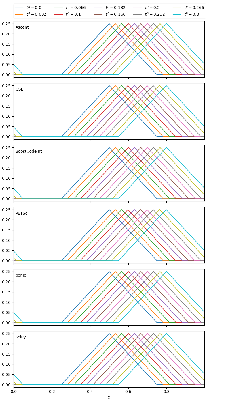
Transport equation#
In this example we would like to solve the following PDE:
with \(t>0\), on the torus \(x\in [0, 1)\), a velocity \(a=1\) and with the initial condition given by:
We choose a first order up-wind scheme to estimate the \(x\) derivative:
and the forward Euler method for time discretization:
where \(\textrm{D}_a\) is the approximation of partial derivative in \(x\) at velocity \(a\). The complet scheme, with \(a>0\), becomes:
In case of \(a=1\) and \(\Delta t = \Delta x\), the scheme gives the exact solution. The explicit Euler method (or forward Euler method) is present in:
Ascent with the name
asc::Eulerodeint with the name
eulerpetsc with the name
TSRK1FEponio with the name
euler
In GSL we need to implement our own driver, and in SciPy to provide a Butcher tableau.
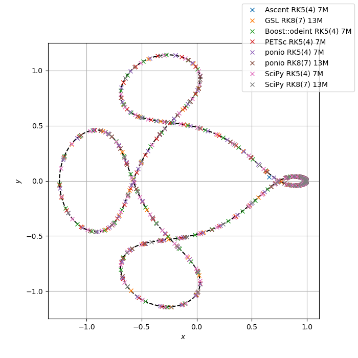
Arenstorf orbit#
We would like to compare some adaptive time step methods with the Arenstorf orbit problem
with initial condition \((x,\dot{x},y,\dot{y})=(0.994, 0, 0, -2.001585106)\), \(r_1\) and \(r_2\) given by
and with parameter \(\mu = 0.012277471\).
First of all, we need to rewrite this problem into a first order derivative equation in time
This is a good example to use an adaptive time step method, because we need a small time step close to the Moon, elsewhere the constraint can be relaxed. For the sake of simplicity we use only native adaptive time step method in each library, it will be:
DOPRI45in Ascentgsl_odeiv2_step_rk8pdin GSLrunge_kutta_dopri5in odeintTSRK5DPin petscrk54_7morrk87_13min ponioRK45orDOP853in SciPy
where DOPRI45, runge_kutta_dopri5, TSRK5DP, rk54_7m or RK45 are the same method, in [DP80] (RK5(4) 7M), see ponio::runge_kutta::rk54_7m_t for more information; and gsl_odeiv2_step_rk8pd, DOP853 and rk87_13m are the same method in [PD81] (RK8(7) 13M) ponio::runge_kutta::rk87_13m_t.