Manage your time loop with Curtiss-Hirschfelder equation

In this example we solve the Curtiss-Hirschfelder equation

\[\dot{y} = k(\cos(t) - y)\]

with stiff parameter \(k=50\) and initial condition \(y(0) = y_0 = 2\). As the name of the \(k\) parameter suggests, this is a stiff equation, so the time step could be constraint by the value of this parameter if we solve this equation with an explicit Runge-Kutta method.

In this case, we need a small time step at the beginning of the simulation, but next, close to the equilibrium we can get larger time step. We can’t do that with ponio::solve() function because we need to change the current step during the simulation. We will use a ponio::solver_range class and access to it with a ponio::time_iterator to manage the time loop.

First of all, we write the problem, in this case the state will be stored into a double, so we don’t specify a state_t for the sake of simplicity.

    double k = 50.;

    auto curtiss_hirschfelder = [=]( double t, double y, double& dy )
    {
        dy = k * ( std::cos( t ) - y );
    };

Next we prepare our simulation, time span, time step, and initial condition

    ponio::time_span<double> const t_span = { 0., 2. }; // begin and end time
    double const dt                       = 0.01;       // time step

    double y_0 = 2.;

ponio::solve function

The standard function to solve a ODE in ponio is with the ponio::solve() function

    auto obs = "curtiss_hirschfelder_solve.txt"_fobs;

    ponio::solve( curtiss_hirschfelder, ponio::runge_kutta::rk_33(), y_0, t_span, dt, obs );

The full example can be found in curtiss_hirschfelder_solve.cpp.

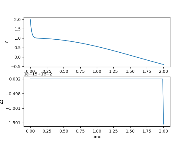
Solution and time step history

A while loop

With the ponio::solve() function we can’t manage solution, or time step. To do this we need a ponio::solver_range

    auto sol_range = ponio::make_solver_range( curtiss_hirschfelder, ponio::runge_kutta::rk_33(), y_0, t_span, dt );

This object is range in C++20 meaning, so we can iterate on it with a ponio::time_iterator object

    auto it_sol    = sol_range.begin();

This kind of iterator can be incremented (++it_sol), and we can access to its stored data with * operator (*it_sol) and get a tuple with \((t^n, y^n, \Delta t^n)\). We can also access with -> operator with it_sol->time for \(t^n\), it_sol->state for \(y^n\) and it_sol->time_step for \(\Delta t^n\). All information contains in this iterator is summarized in the following diagram:

Summarize of time_iterator class

To manage the time loop we write a while loop

    while ( it_sol->time < 2. )
    {
        obs( it_sol->time, it_sol->state, it_sol->time_step );

        // pseudo adaptive time-step method
        if ( it_sol->time < 0.5 )
        {
            ++it_sol;
        }
        else
        {
            it_sol->time_step = 0.05;
            ++it_sol;
        }
    }
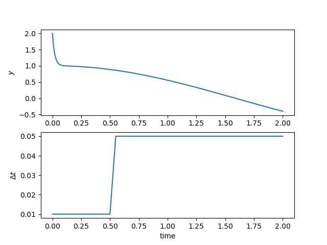
    obs( it_sol->time, it_sol->state, 2. - it_sol->time ); // to save iteration where it_sol->time == tf

We can access in read and write to data in iterator.

The full example can be found in curtiss_hirschfelder_while.cpp.

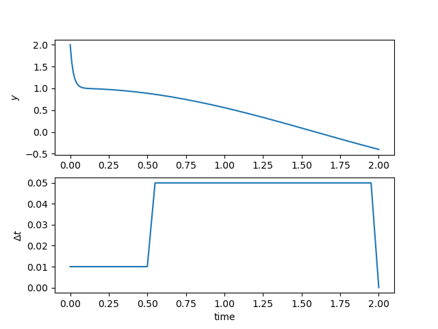
Solution and time step history

A for loop

Like for a while loop, we need to build a ponio::solver_range and iterate on it by using a range-based for loop.

    auto sol_range = ponio::make_solver_range( curtiss_hirschfelder, ponio::runge_kutta::rk_33(), y_0, t_span, dt );

If you want to modify the tuple \((t^n, y^n, \Delta t^n)\) we need a reference :

for ( auto& ui : sol_range )
// ...

Else we can just use a value

for ( auto ui : sol_range )
// ...

The complet for loop is the following

    for ( auto& ui : sol_range )
    {
        obs( ui.time, ui.state, ui.time_step );

        if ( ui.time < 0.5 )
        {
            ui.time_step = 0.01;
        }
        else
        {
            ui.time_step = 0.05;
        }
    }

The full example can be found in curtiss_hirschfelder_for.cpp.

Solution and time step history