Very first steps with Lorenz system#
In this example, we present how to solve Lorenz system, step by step, with ponio library. The Lorenz system is the following
with initial condition \((x,y,z)=(1,1,1)\) and parameter \(\sigma=10\), \(\rho=28\) and \(\beta=\frac{8}{3}\). We present in this section how to solve it with an explicit Runge-Kutta method, a Lawson method, a diagonal implicit Runge-Kutta method and a splitting method.
Explicit Runge-Kutta solver#
In this section we solve this problem with a classical Runge-Kutta method. First of all we need to rewrite the problem as \(\dot{u} = f(t, u)\), here we choose \(u = (x, y, z)\)
next we choose a data structure to store state \(u\), for the sake of simplicity we chose the STL container std::valarray<double>:
17 using state_t = std::valarray<double>;
Now we can write \(f:t, u\mapsto f(t,u)\) as a lambda function:
19    double sigma = 10., rho = 28., beta = 8. / 3.;
20
21    auto lorenz = ponio::make_simple_problem(
22        [=]( double /* t */, state_t&& u ) -> state_t
23        {
24            double dt_u0 = sigma * ( u[1] - u[0] );
25            double dt_u1 = rho * u[0] - u[1] - u[0] * u[2];
26            double dt_u2 = u[0] * u[1] - beta * u[2];
27
28            return { dt_u0, dt_u1, dt_u2 };
29        } );
ponio library provides interface for a function \(f\) defined in this way, but we need to embedded it in a ponio::simple_problem (see the call of ponio::solve() function). Next we define the initial condition to \(u_0 = (1, 1, 1)\), the initial and final time in a time span (here between \(0\) and \(20\)) the time step \(\Delta t = 0.01\) and solve with all this parameters with a classical RK(4,4): ponio::runge_kutta::rk_44_t.
Note
List of all explicit Runge-Kutta methods can be found in the algorithms section.
31    state_t const u0 = { 1., 1., 1. };
32
33    ponio::time_span<double> const tspan = { 0., 20. };
34    double const dt                      = 0.01;
35
36    ponio::solve( lorenz, ponio::runge_kutta::rk_44(), u0, tspan, dt, "lorenz_rk_pb.txt"_fobs );
In the last line we call ponio::solve() function, with a observer::file_observer to store the output in lorenz_rk_pb.txt text file.
Note
To use the _fobs literal you need to using the correct namespace
using namespace ponio::observer; // to use _fobs litteral
The full example can be found in lorenz_rk_pb.cpp.
You can compile this example
$CXX -std=c++20 -I PONIO_INCLUDE lorenz_rk_pb.cpp -o lorenz_rk_pb
or with a cmake like in ponio-gallery repository.
The output looks like this
0 1 1 1  0.01000000000000000021
0.01000000000000000021 1.01256719107361115 1.259917798945274114 0.9848909717916053408  0.01000000000000000021
0.02000000000000000042 1.048823709708956997 1.52399713132260084 0.9731142198764850537  0.01000000000000000021
0.02999999999999999889 1.107208854295661515 1.798309889742135237 0.9651589513000615739  0.01000000000000000021
0.04000000000000000083 1.18686801666034647 2.088540142206162464 0.9617372249104277904  0.01000000000000000021
with in the first column the current time, the last one the current time step and between all compostant of current state. We can plot it using NumPy and Matplotlib with the following example script
import numpy as np
import matplotlib.pyplot as plt

data = np.loadtxt("lorenz_rk_pb.txt")
ax = plt.figure().add_subplot(projection='3d')
x, y, z = data[:,1], data[:, 2], data[:, 3]
ax.plot( x, y, z )
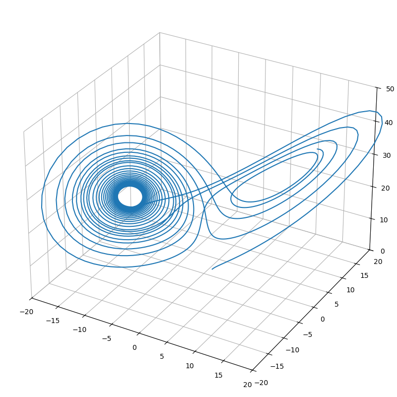
Lorenz attractor solved by RK(4, 4) method#
Like many other library, ponio library provides an interface with a function \(f\) which takes the output by reference to provides extra-allocation:
now the ponio::solve() function can takes this lambda without underlying it in a class:
0.3100000000000001088 17.67463919318145571 26.88360583967070738 30.11213496677726198 0.01000000000000000021
The full example can be found in lorenz_rk.cpp.
You can compile this example
$CXX -std=c++20 -I PONIO_INCLUDE lorenz_rk.cpp -o lorenz_rk
Lawson solver#
In this section we propose to solve the Lorenz equations with a Lawson method. First of all we need to rewrite the system with a linear and non-linear part, as \(\dot{u} = Lu + N(t, u)\), with \(u=(x, y, z)\)
A Lawson method needs to compute an exponential of the linear part, but the ponio library doesn’t provide linear algebra, and even less an exponential function for matrices. For that you can use Eigen 3, so the definition of type of state \(u^n\) changes into
18    using vector_type = Eigen::Vector<double, 3>;
19    using matrix_type = Eigen::Matrix<double, 3, 3>;
20
21    using state_t = vector_type;
Now we can write the linear part \(L\) and non-linear part \(N:t, u\mapsto N(t,u)\), and store them into a ponio::lawson_problem
23    double sigma = 10., rho = 28., beta = 8. / 3.;
24
25    auto L = matrix_type{
26        {-sigma, sigma, 0    },
27        { rho,   -1,    0    },
28        { 0,     0,     -beta}
29    };
30    auto N = [=]( double, auto&& u, state_t& du )
31    {
32        du[0] = 0.;
33        du[1] = -u[0] * u[2];
34        du[2] = u[0] * u[1];
35    };
36    auto lorenz = ponio::make_lawson_problem( L, N );
The ponio::lawson_problem builds in the emphasize line provides an interface which can be use by a classical explicit Runge-Kutta method or a Lawson method.
We have to define the exponential function which takes a matrix and return a matrix
39    auto m_exp = []( matrix_type const& A ) -> matrix_type
40    {
41        return A.exp();
42    };
We can also define your own exponential function if you know the analytic form of the result of \(\exp(\tau L)\) with \(\tau = c_j\Delta t\).
The call of function ponio::solve() doesn’t change
44    state_t const u0 = { 1., 1., 1. };
45
46    ponio::time_span<double> const tspan = { 0., 20. };
47    double const dt                      = 0.01;
48
49    ponio::solve( lorenz, ponio::runge_kutta::lrk_44( m_exp ), u0, tspan, dt, "lorenz_lrk.txt"_fobs );
We use the Lawson method given by the underlying RK(4,4) method: ponio::runge_kutta::lrk_44_t.
Note
List of all Lawson methods can be found in the algorithms section.
The full example can be found in lorenz_lrk.cpp.
Diagonal implicit Runge-Kutta solver#
In this section we solve this problem with an implicit Runge-Kutta method. We keep the problem with the form \(\dot{u} = f(t,u)\) but we need to provide the Jacobian function for the Newton method at each stage.
Because we will use linear algebra, we use Eigen 3 to define the state
19    using vector_type = Eigen::Vector<double, 3>;
20    using matrix_type = Eigen::Matrix<double, 3, 3>;
21
22    using state_t = vector_type;
Now we define the function and its Jacobian defined by
and create a ponio::implicit_problem
24    double sigma = 10., rho = 28., beta = 8. / 3.;
25
26    auto f = [=]( double /* t */, auto const& u, state_t& du )
27    {
28        du[0] = sigma * ( u[1] - u[0] );
29        du[1] = rho * u[0] - u[1] - u[0] * u[2];
30        du[2] = u[0] * u[1] - beta * u[2];
31    };
32    auto jac_f = [=]( double, state_t const& u ) -> matrix_type
33    {
34        return matrix_type( {
35            {-sigma,      sigma, 0    },
36            { rho - u[2], -1,    -u[0]},
37            { u[1],       u[0],  -beta}
38        } );
39    };
40    auto lorenz = ponio::make_implicit_problem( f, jac_f );
Finally we can solve the problem with the same lines of previous solver
42    state_t const u0 = { 1., 1., 1. };
43
44    ponio::time_span<double> const tspan = { 0., 20. };
45    double const dt                      = 0.01;
46
47    ponio::solve( lorenz, ponio::runge_kutta::dirk34(), u0, tspan, dt, "lorenz_dirk.txt"_fobs );
We use the DIRK(3, 4) method: ponio::runge_kutta::dirk34_t().
Note
List of all DIRK methods can be found in the algorithms section.
The full example can be found in lorenz_dirk.cpp.
Splitting solver#
For the splitting method, we split the problem into multiple parts. We chose here 3 parts, but ponio can take any number of part for the splitting. We choose arbitrarily the following splitting
The splitting is defined as
for the Lie splitting method, and
for the Strang splitting method, where \(\varphi_{\tau}^{[j]}\) is a numerical approximation of the step \(j\) between \(0\) and \(\tau\) with a specific time step \(\delta t < \tau\). For more information see splitting section.
For the sake of simplicity, we solve each step with a explicit Runge-Kutta method, but you can use any other solver (even a splitting method!).
Like other solver, first of all we define our state
18 using state_t = std::valarray<double>;
Next we define the three function to represent \(\varphi^{[0]}\), \(\varphi^{[1]}\), \(\varphi^{[2]}\)
20    double sigma = 10., rho = 28., beta = 8. / 3.;
21
22    auto phi_0 = [=]( double /* t */, auto&& u, state_t& du )
23    {
24        du[0] = sigma * u[1];
25        du[1] = rho * u[0];
26        du[2] = u[0] * u[1];
27    };
28    auto phi_1 = [=]( double /* t */, auto&& u, state_t& du )
29    {
30        du[0] = -sigma * u[0];
31        du[1] = -u[1];
32        du[2] = -beta * u[2];
33    };
34    auto phi_2 = [=]( double /* t */, auto&& u, state_t& du )
35    {
36        du[0] = 0;
37        du[1] = -u[0] * u[2];
38        du[2] = 0;
39    };
40    auto lorenz = ponio::make_problem( phi_0, phi_1, phi_2 );
Now we create a tuple of algorithms with ponio::splitting::lie::make_lie_tuple() or ponio::splitting::strang::make_strang_tuple() for respectively a Lie splitting method or Strang splitting method. In ponio their is also an adaptive time stepping Strang splitting method with ponio::splitting::strang::make_adaptive_strang_tuple().
42    auto strang = ponio::splitting::make_strang_tuple( std::make_pair( ponio::runge_kutta::rk_44_38(), 0.01 ),
43        std::make_pair( ponio::runge_kutta::rk_44(), 0.005 ),
44        std::make_pair( ponio::runge_kutta::rk_44_ralston(), 0.0005 ) );
We have to select an algorithm for each step of splitting method, and specify a time step (smaller than splitting time step), in this case we choose 3 different Runge-Kutta methods of order 4 with 4 stages:
A first RK(4,4) 3/8 rule:
ponio::runge_kutta::rk_44_38_t, with a time step \(\delta t = 0.01\) (equals to the splitting time step)A second RK(4,4), classical one:
ponio::runge_kutta::rk_44_t, with a time step \(\delta t = 0.005\)A third RK(4,4), from Ralston:
ponio::runge_kutta::rk_44_ralston_t, with a time step \(\delta t = 0.0005\)
For each algorithm we specify a time step to solve each \(\varphi^{[i]}\).
For a Lie splitting this code become
auto lie = ponio::splitting::make_lie_tuple( std::make_pair( ponio::runge_kutta::rk_44_38(), 0.01 ),
      std::make_pair( ponio::runge_kutta::rk_44(), 0.005 ),
      std::make_pair( ponio::runge_kutta::rk_44_ralston(), 0.0005 ) );
Finally we call ponio::solve() function, as previous solver
46    state_t const u0 = { 1., 1., 1. };
47
48    ponio::time_span<double> const tspan = { 0., 20. };
49    double const dt                      = 0.01;
50
51    ponio::solve( lorenz, strang, u0, tspan, dt, "lorenz_split.txt"_fobs );
The full example can be found in lorenz_split.cpp.
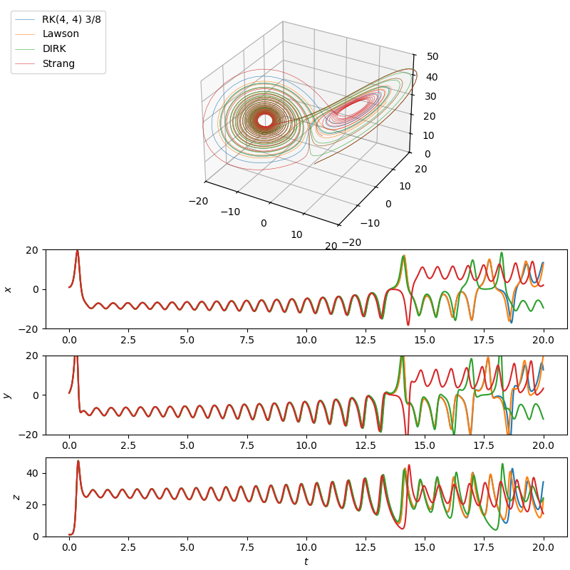
Lorenz attractor solved by each presented methods#