Examples

The following table gives an overview over all examples.

Section	Brief Description	File
Arenstorf orbit	This example shows how to use multiple adaptive time step methods	arenstorf.cpp
Brownian movement	This example shows how to use random in an ODE	brownian.cpp
Brusselator equations	The chemistry example of Brusselator (2 equations model)	brusselator.cpp
Brusselator equations with DIRK method	This example shows hos to use DIRK methods	brusselator_dirk.cpp
Curtiss-Hirschfelder equation	This example shows how to use range and iterators on solution	curtiss_hirschfelder.cpp
Curtiss-Hirschfelder equation with expRK method	This example shows how to use exponential Runge-Kutta methods	curtiss_hirschfelder_exprk.cpp
Exponential function	This example is the simplest example	exp.cpp
Exponential function with exact solver	An example of splitting and exact solver	exp_splitting.cpp
Heat model	The classical heat equation solving with RKC2 method	heat.cpp
ROCK method	This example shows how to use ROCK2 and ROCK4 methods	heat_rock.cpp
Samurai is hot	This example shows how to coupling ponio and samurai	heat_samurai.cpp
Lorenz equations	The chaotic system example of Lorenz equations	lorenz.cpp
Lorenz equations with multiple methods	This example shows how to use splitting methods and Lawson methods	lorenz_tuto.cpp
Lorenz equations with all methods	This example shows how to use all methods (except expRK)	lorenz_all.cpp
Lotka-Volterra model	The classical predator–prey model of Lotka-Volterra	lotka_volterra.cpp
Nagumo equation	Example of a traveling wave	nagumo.cpp
Pendulum equation	The classical pendulum equation	pendulum.cpp
Belousov Zhabotinsky	Solves Belousov-Zhabotinsky equations with PIROCK method	belousov_zhabotinsky_pirock.cpp
Belousov Zhabotinsky in 2D	Solves Belousov-Zhabotinsky equations with PIROCK method in 2D	bz_2d_pirock.cpp

To lunch examples, in the main directory of ponio run:

cmake . -B build -DBUILD_DEMOS=ON

Eventually to get examples with samurai run:

cmake . -B build -DBUILD_DEMOS=ON -DBUILD_SAMURAI_DEMOS=ON

and

cd build

next you can compile an example with

make AN_EXAMPLE

you could also launch the Python script which launch the example and display results

make AN_EXAMPLE_visu

or

make visu_AN_EXAMPLE

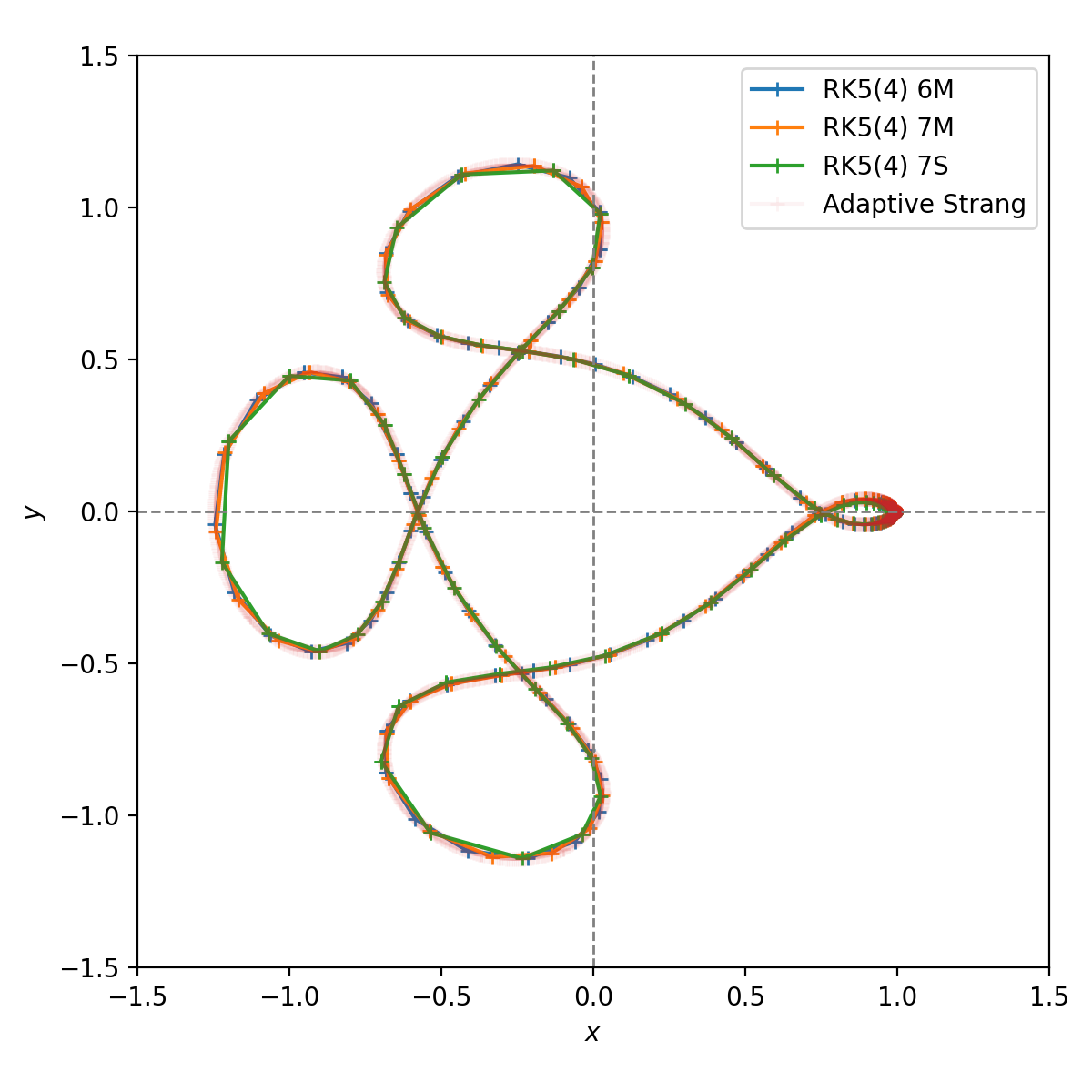
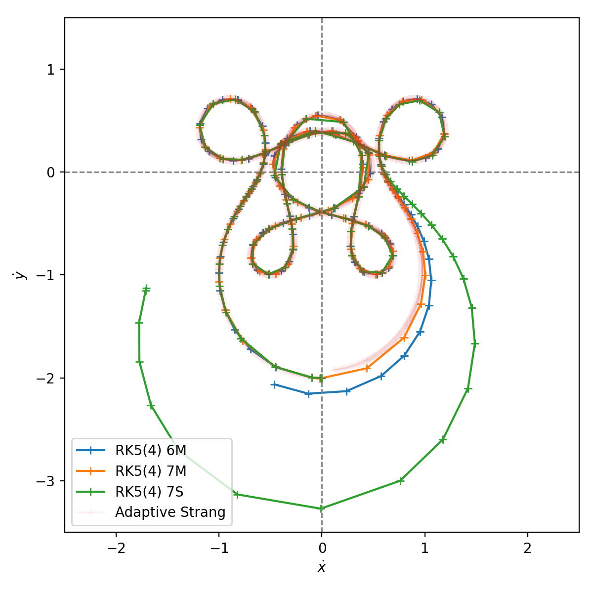
Arenstorf orbit

The system of differential equations for the Arenstorf orbit are:

\[\begin{split}\begin{cases} \ddot{x} &= x + 2\dot{y} - \frac{1-\mu}{r_1^3}(x+\mu) - \frac{\mu}{r_2^3}(x-1+\mu) \\ \ddot{y} &= y - 2\dot{x} - \frac{1-\mu}{r_1^3}y - \frac{\mu}{r_2^3}y \end{cases}\end{split}\]

where

\[r_1 = \sqrt{(x+\mu)^2 + y^2},\quad r_2 = \sqrt{(x-1+\mu)^2 + y^2}\]

parameter \(\mu=0.012277471\) and the initial condition gives by:

\[x(0) = 0.994,\quad \dot{x}(0) = 0,\quad y(0) = 0,\quad \dot{y}(0) = -2.00158510637908252240537862224\]

To solve this kind of problem with ponio, first of all you should rewrite it as the form: \(\dot{u} = f(t, u)\), here we classically take

\[\begin{split}u = \begin{pmatrix} x \\ y \\ \dot{x} \\ \dot{y} \end{pmatrix}\end{split}\]

So we have:

\[\begin{split}\dot{u} = \begin{pmatrix} \dot{x} \\ \dot{y} \\ \ddot{x} \\ \ddot{y} \end{pmatrix} = \begin{pmatrix} \dot{x} \\ \dot{y} \\ x + 2\dot{y} - \frac{1-\mu}{r_1^3}(x+\mu) - \frac{\mu}{r_2^3}(x-1+\mu) \\ y - 2\dot{x} - \frac{1-\mu}{r_1^3}y - \frac{\mu}{r_2^3}y \end{pmatrix} = f(t, u)\end{split}\]

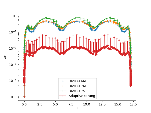
In this example we solve this system with some explicit adaptive time step methods from Dormand, J.R., Prince, P.J., A family of embedded Runge-Kutta formulae (1980) Journal of Computational and Applied Mathematics

Arenstorf orbit	Arenstorf velocity

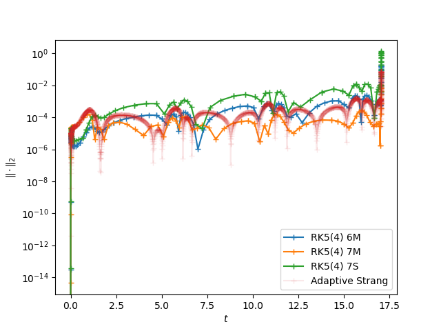
Time step history	Error over time

All example in arenstorf.cpp, and run

make arenstorf_visu

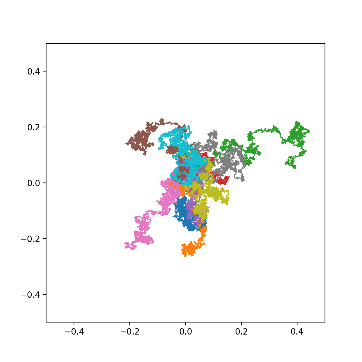
Brownian movement

We write a simple Brownian movement

\[\begin{split}\begin{cases} \dot{x} = X(t) \\ \dot{y} = Y(t) \end{cases}\end{split}\]

where \(X(t)\) and \(Y(t)\) are random variable (juste a std::rand at each iteration).

Some Brownian movement in 2D

All example in brownian.cpp, and run

make brownian_visu

Brusselator equations

The Brusselator is a model of periodic chemical reaction. We present the version ODE with two species

\[\begin{split}\begin{cases} \dot{x} &= m_a - (m_b + 1)x + x^2y \\ \dot{y} &= m_b x - x^2y \end{cases}\end{split}\]

We solve this model with a hight order explicit Runge-Kutta method: RK(8, 6).

Brusselator concentration	Brusselator concentration in phase space

All example in brusselator.cpp, and run

make brusselator_visu

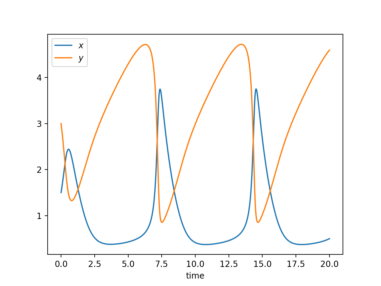
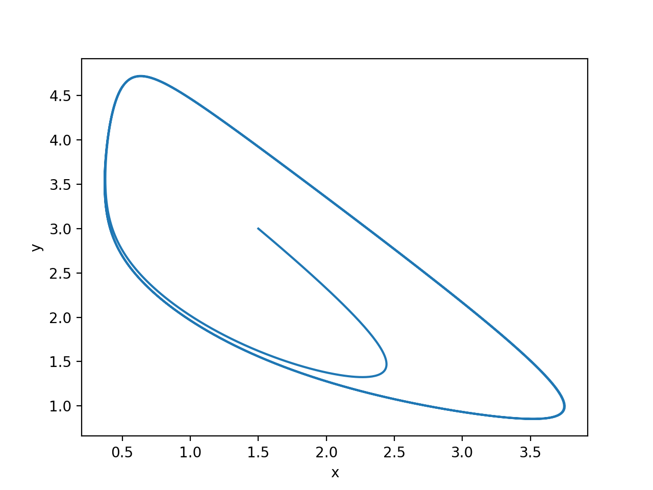
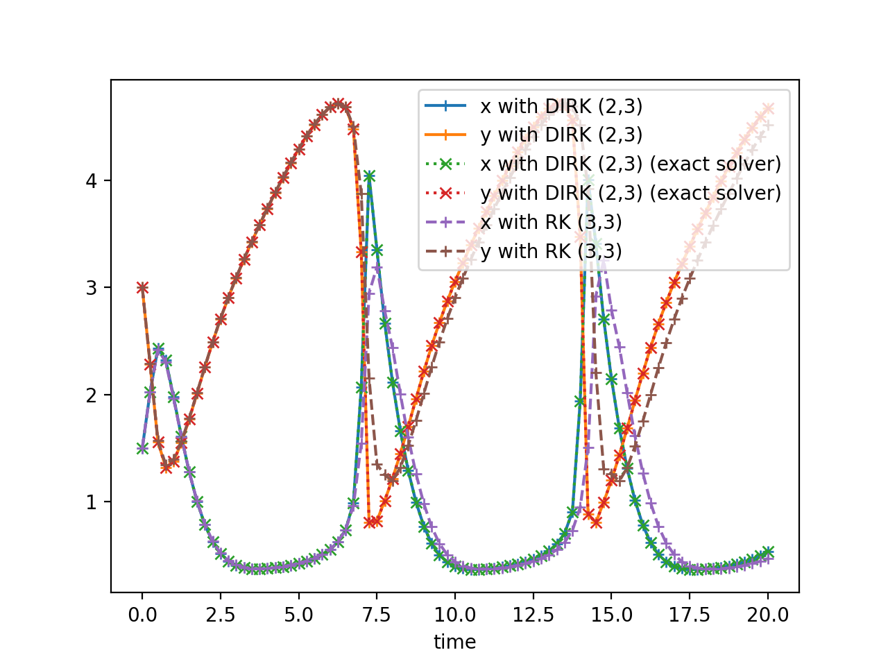
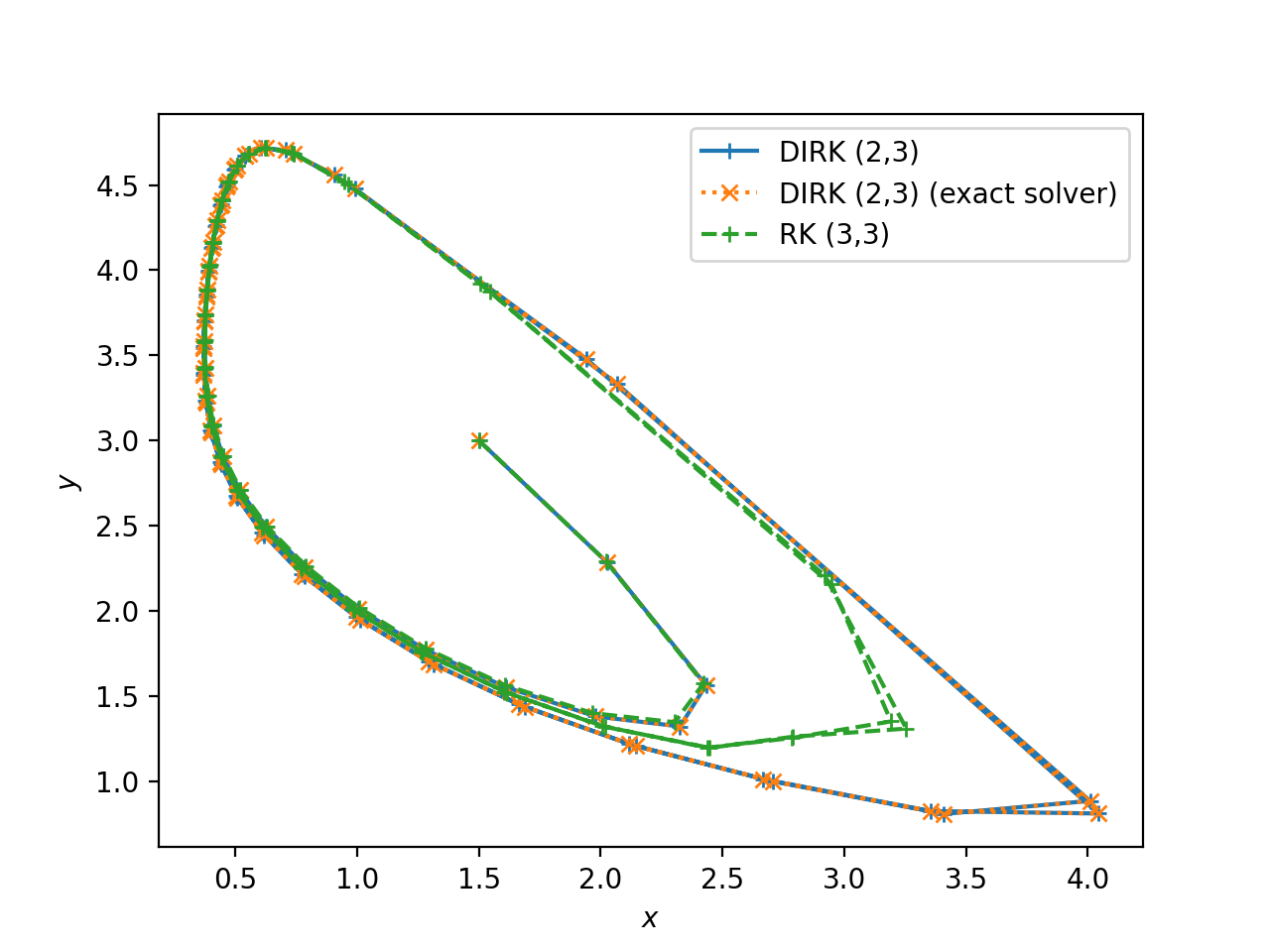
Brusselator equations with DIRK method

The Brusselator is a model of periodic chemical reaction. We present the version ODE with two species

\[\begin{split}\begin{cases} \dot{x} &= m_a - (m_b + 1)x + x^2y \\ \dot{y} &= m_b x - x^2y \end{cases}\end{split}\]

In this example we choose to solve the model with a diagonal-implicit Runge-Kutta method. The problem object has to be an ponio::implicit_problem and we need to compute the Jacobian matrix and proposes some linear algebra routines. For that we use Eigen library.

If state_t is floating point, a Eigen vector or a samurai field, ponio provides functions to solve implicit problems. In all cases, you can specify your own linear algebra object that contains a solver method (see lin_alg_2_2 structure), that takes a matrix \(A\) (same type as the returns type of jacobian gives to ponio::implicit_problem) and a vector \(b\) (same type as state_t) and return the solution of the linear problem

\[Ax = b.\]

Brusselator concentration	Brusselator concentration in phase space

All example in brusselator_dirk.cpp, and run

make brusselator_dirk_visu

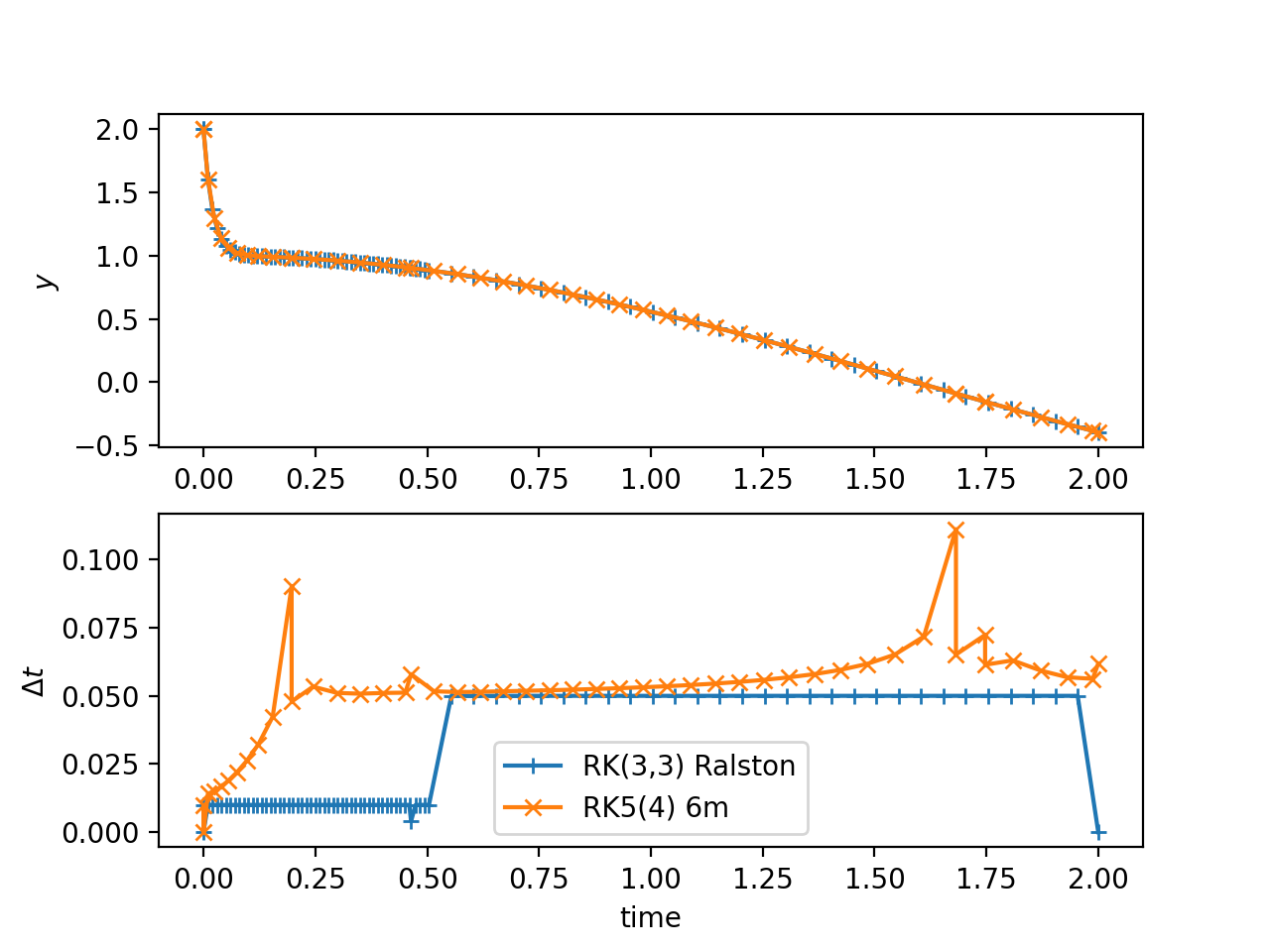
Curtiss-Hirschfelder equation

A classical stiff problem is the Curtiss-Hirschfelder equation

\[\dot{y} = k(\cos(t) - y)\]

with \(k>1\) and \(y(0) = y_0\). We choose \(k = 50\) and \(y_0 = 2\).

In this example we present how to control time loop with a ponio::solver_range. You can do it with an iterator on this range with :

auto sol_range = ponio::make_solver_range( ... );

and iterate over this range with a classical iterator with:

for ( auto it = sol_range.begin(); it < sol_range.end(); ++it )
{
  // ...
  // current time : it->time
  // current state : it->state
  // current time step : it->time_step
}

or with a range-based for loop:

for ( auto ui : sol_range )
{
  // ...
}

Only in the first case you can control time step before increment (with your adaptive time step heuristic) with modification of it->time_step data member.

Curtiss-Hirschfelder solution

All example in curtiss_hirschfelder.cpp, and run

make curtiss_hirschfelder_visu

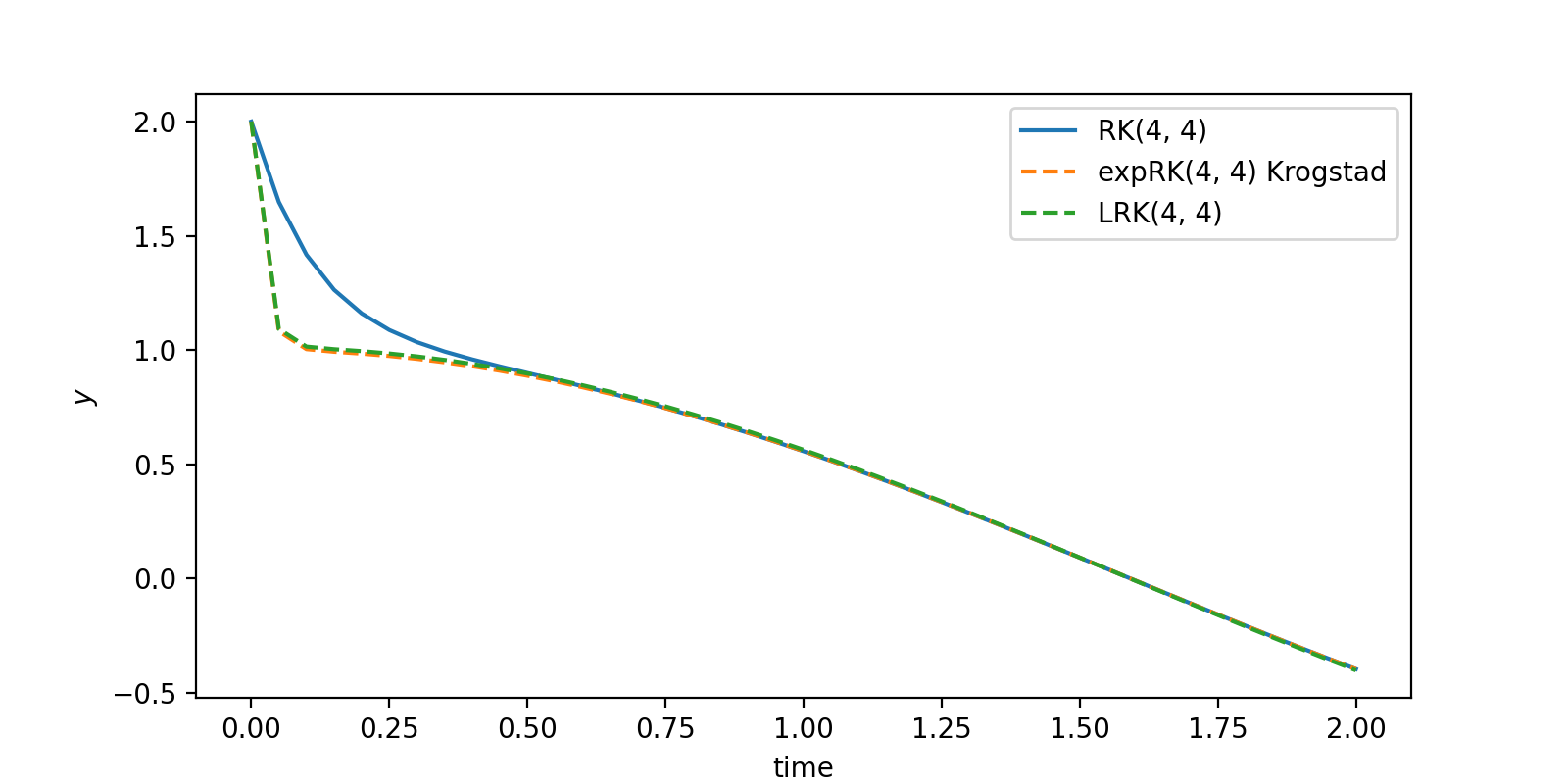
Curtiss-Hirschfelder equation with expRK method

A classical stiff problem is the Curtiss-Hirschfelder equation

\[\dot{y} = k(\cos(t) - y)\]

with \(k>1\) and \(y(0) = y_0\). We choose \(k = 50\) and \(y_0 = 2\).

In this example we solve the equation with Krogstad method (an exponential Runge-Kutta method), and LRK(4, 4) method (a Lawson method). In both methods, you need to define a ponio::lawson_problem with a linear and non-linear part. We choose the linear part \(-k\) and the non-linear part as \(N:t, y\mapsto k\cos(t)\). Exponential Runge-Kutta methods and Lawson methods are build to solve exactly the linear part when the non-linear part goes to 0.

Curtiss-Hirschfelder solution

All example in curtiss_hirschfelder_exprk.cpp, and run

make curtiss_hirschfelder_exprk_visu

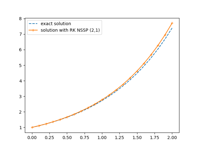
Exponential function

In this example we solve the simplest differential equation:

\[\dot{y} = y\]

with \(y(0) = 1\). After a lot of calculus we can find the exact solution \(y(t) = e^t\), or we can approximate it with RK NSSP (2, 1) method.

Exponential function

All example in exp.cpp, and run

make exp_visu

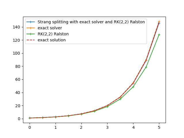
Exponential function with exact solver

In this example we solve the simplest differential equation:

\[\dot{y} = \lambda y + (1-\lambda )y\]

with \(y(0) = 1\) and \(\lambda = 0.3\). In this example we solve this equation with:

• a Strang splitting method with \(f_1:(t,y)\mapsto \lambda y\) (which is solved exactly), and \(f_2:(t,y)\mapsto (1-\lambda)y\) (which is solved with a RK(2,2) Raslton).

• an exact solver \(\phi:(f,t,u,\Delta t)\mapsto e^{\Delta t}u\).

• a RK(2,2) Ralston method.

Exponential function

All example in exp_splitting.cpp, and run

make exp_splitting_visu

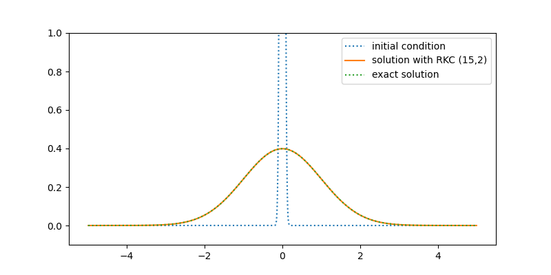
Heat model

In this example we propose to solve a PDE, the heat equation in 1D

\[\partial_t u = -\partial_{xx} u\]

with the initial condition gives by the fundamental solution of head equation at time \(t=0.001\) given by:

\[u(t, x) = \frac{1}{2\sqrt{\pi t}} e^{-\frac{x^2}{4t}}\]

In ponio, the state_t should propose arithmetic operations as addition and multiplication by a scalar (of type value_t). For the sake of simplicity, we use in the example a std::valarray<double>.

The heat equation is quite complicated to solve with an explicit Runge-Kutta method but we do it with a extended stability method with the Runge-Kutta Chebyshev of order 2. In ponio you could choose the number of stages of this method : ponio::runge_kutta::explicit_rkc2<15>() (for 15 stages).

Solution of heat equation

All example in heat.cpp, and run

make heat_visu

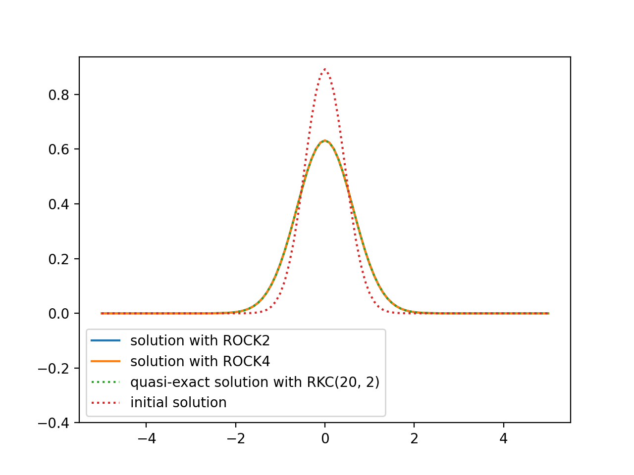
ROCK method

In this example we propose to solve a PDE, the heat equation in 1D

\[\partial_t u = -\partial_{xx} u\]

with the initial condition gives by the fundamental solution of head equation at time \(t=0.001\) given by:

\[u(t, x) = \frac{1}{2\sqrt{\pi t}} e^{-\frac{x^2}{4t}}\]

In ponio, the state_t should propose arithmetic operations as addition and multiplication by a scalar (of type value_t). For the sake of simplicity, we use in the example a std::valarray<double>.

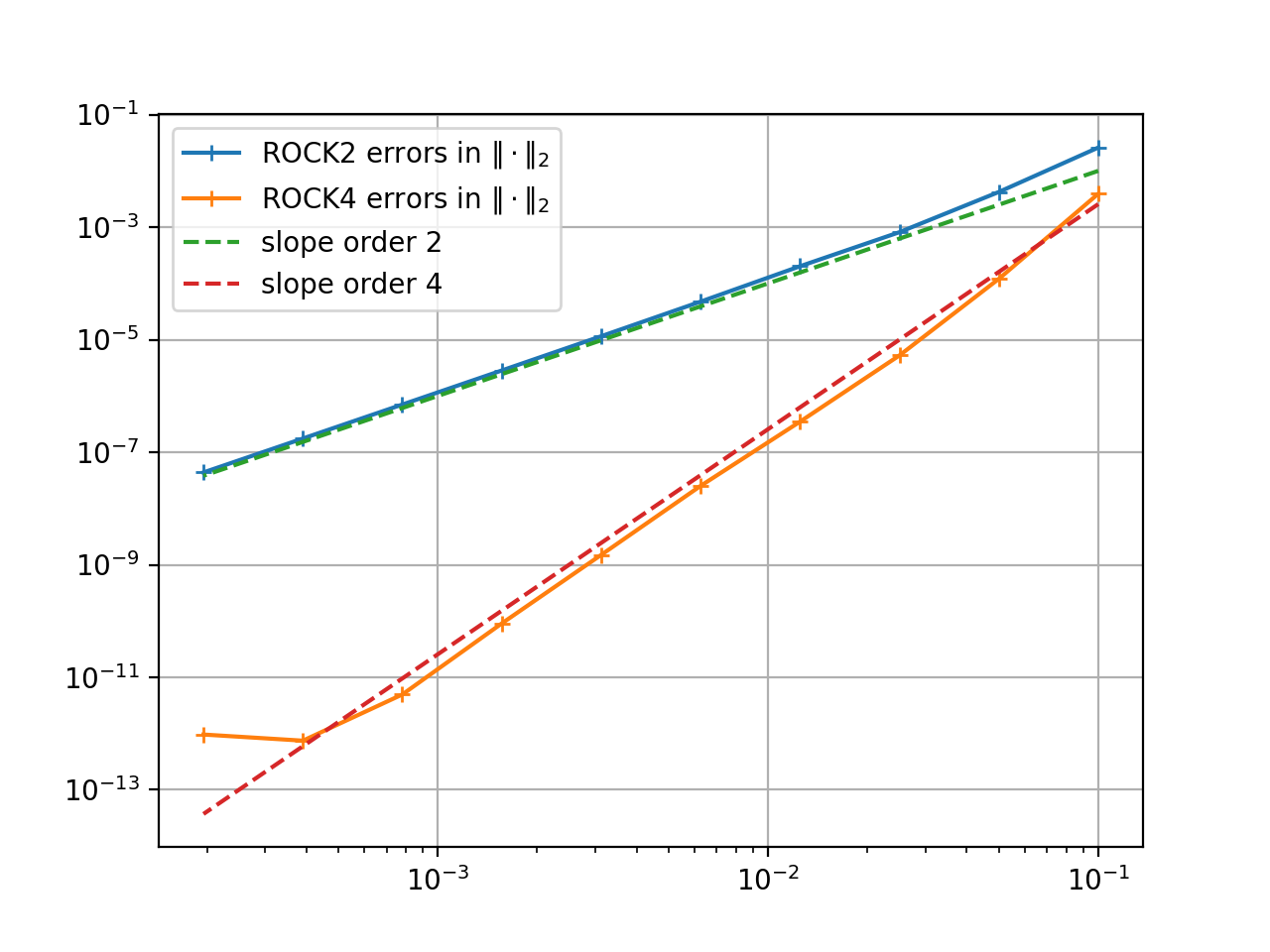
An optimization of RKC2 is the ROCK2 method from Abdulle, A., Medovikov, A. Second order Chebyshev methods based on orthogonal polynomials. Numer. Math (2001), and its extension to order 4, ROCK4 method presented in Abdulle, A. Fourth Order Chebyshev Methods with Recurrence Relation. SIAM Journal on Scientific Computing (2002).

Solution of heat equation	Mesure of order of ROCK2 and ROCK4

All example in heat_rock.cpp, and run

make heat_rock_visu

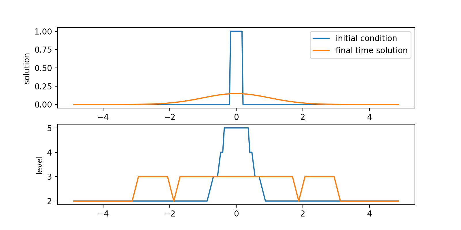
Samurai is hot

This example needs to activate -DBUILD_SAMURAI_DEMOS=ON

In this example we propose to solve a PDE, the heat equation in 1D

\[\partial_t u = -\partial_{xx} u\]

with the initial condition gives by the fundamental solution of head equation at time \(t=0.001\) given by:

\[u(t, x) = \frac{1}{2\sqrt{\pi t}} e^{-\frac{x^2}{4t}}\]

In this example we coupling the mesh refinement library samurai with ponio.

Solution of heat equation with levels of adaptive mesh

All example in heat_samurai.cpp, and run

make heat_samurai_visu

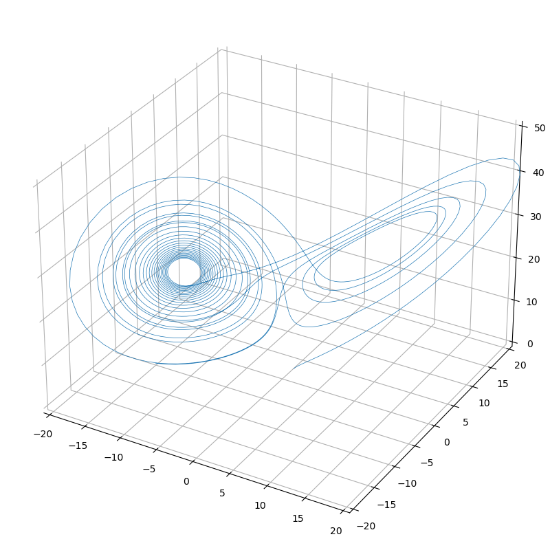
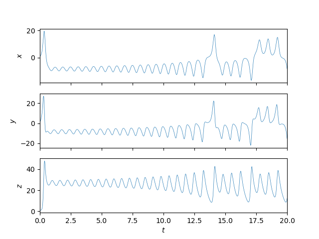
Lorenz equations

The classical chaotic system example of Lorenz equations

\[\begin{split}\begin{cases} \dot{x} &= \sigma (y - x) \\ \dot{y} &= \rho x - y - xz \\ \dot{z} &= xy - \beta z \end{cases}\end{split}\]

Solution in 3D	Solution by composant

All example in lorenz.cpp, and run

make lorenz_visu

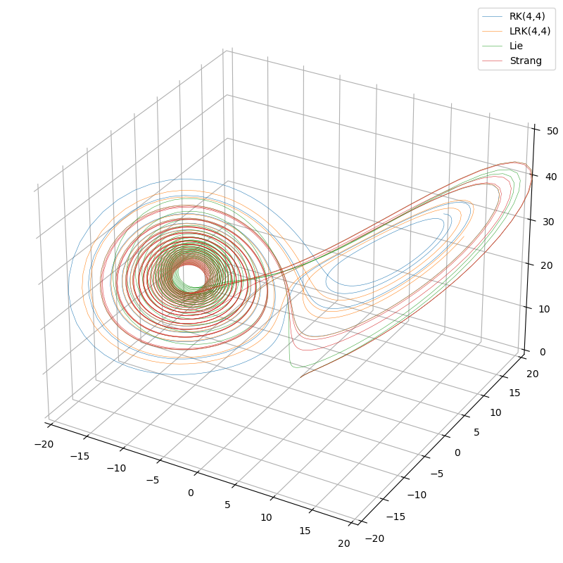
Lorenz equations with multiple methods

The classical chaotic system example of Lorenz equations

\[\begin{split}\begin{cases} \dot{x} &= \sigma (y - x) \\ \dot{y} &= \rho x - y - xz \\ \dot{z} &= xy - \beta z \end{cases}\end{split}\]

Solution in 3D	Solution by composant

All example in lorenz_tuto.cpp, and run

make lorenz_tuto_visu

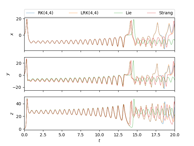
Lorenz equations with all methods

The classical chaotic system example of Lorenz equations

\[\begin{split}\begin{cases} \dot{x} &= \sigma (y - x) \\ \dot{y} &= \rho x - y - xz \\ \dot{z} &= xy - \beta z \end{cases}\end{split}\]

Solution in 3D

All example in lorenz_all.cpp, and run

make lorenz_all_visu

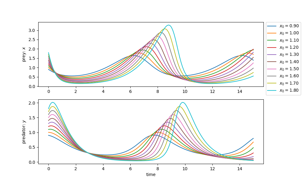
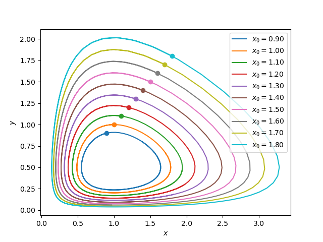
Lotka-Volterra model

The classical predator–prey model of Lotka-Volterra:

\[\begin{split}\begin{cases} \dot{x} = \alpha x - \beta xy \\ \dot{y} = \delta xy - \gamma y \end{cases}\end{split}\]

with parameters \(\alpha=\frac{2}{3}\), \(\beta=\frac{4}{3}\), \(\gamma = \delta = 1\), and with the initial condition \((x, y) = (x_0, x_0)\), with different values of \(x_0\).

Prey predator history	Solution in phase space

All example in lotka_volterra.cpp, and run

make lotka_volterra_visu

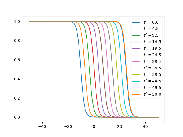
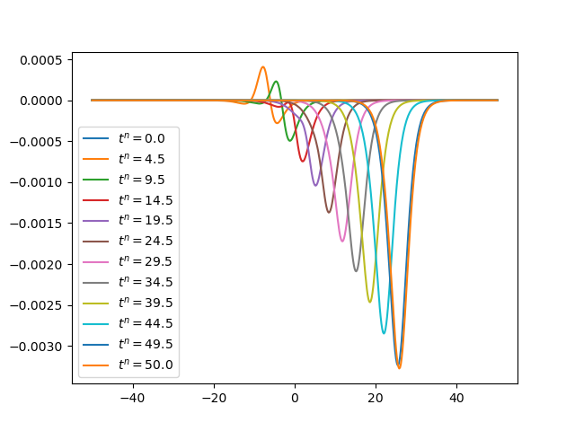
Nagumo equation

The Nagumo equation is a propagation of a traveling wave

\[\partial_t u = d \partial_{xx}u + ku^2(1-u)\]

with parameter \(k=1\), \(d=1\), with the initial solution given by exact solution to time \(t=0\):

\[u(t, x) = \frac{\exp(c(x - x_0 - vt))}{1 + \exp(c(x-x_0 - vt))}\]

where

\[v = \frac{1}{\sqrt{2}}\sqrt{kd},\quad c = -\frac{1}{\sqrt{2}}\sqrt{\frac{k}{d}},\quad x_0 = -10.\]

Solution with RKC(20, 2)	Absolute error

All example in nagumo.cpp, and run

make nagumo_visu

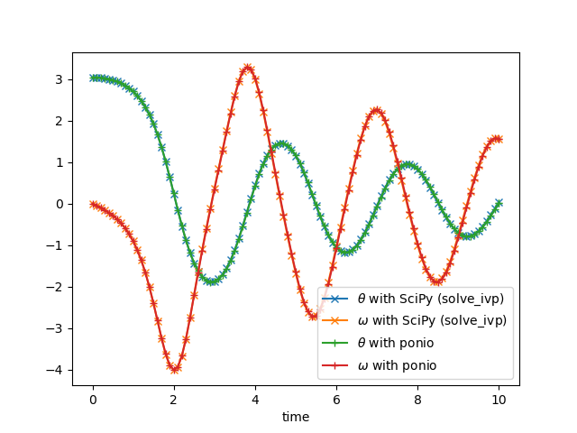
Pendulum equation

The second order differential equation for the angle \(\theta\) of a pendulum acted on by gravity with friction can be written:

\[\ddot{\theta} + b\dot{\theta} + c\sin(\theta) = 0\]

where \(b\) and \(c\) are positive constants, we take \(b=0.25\), \(c=5.0\). As Arenstorf orbit, we have to rewrite problem as \(\dot{u} = f(t, u)\) :

\[\begin{split}\partial_t \begin{pmatrix} \theta \\ \omega \end{pmatrix} = \begin{pmatrix} \omega \\ -b\omega - c\sin(\theta) \end{pmatrix}\end{split}\]

Pendulum equation (solved with RK (4,4))

All example in pendulum.cpp, and run

make pendulum_visu

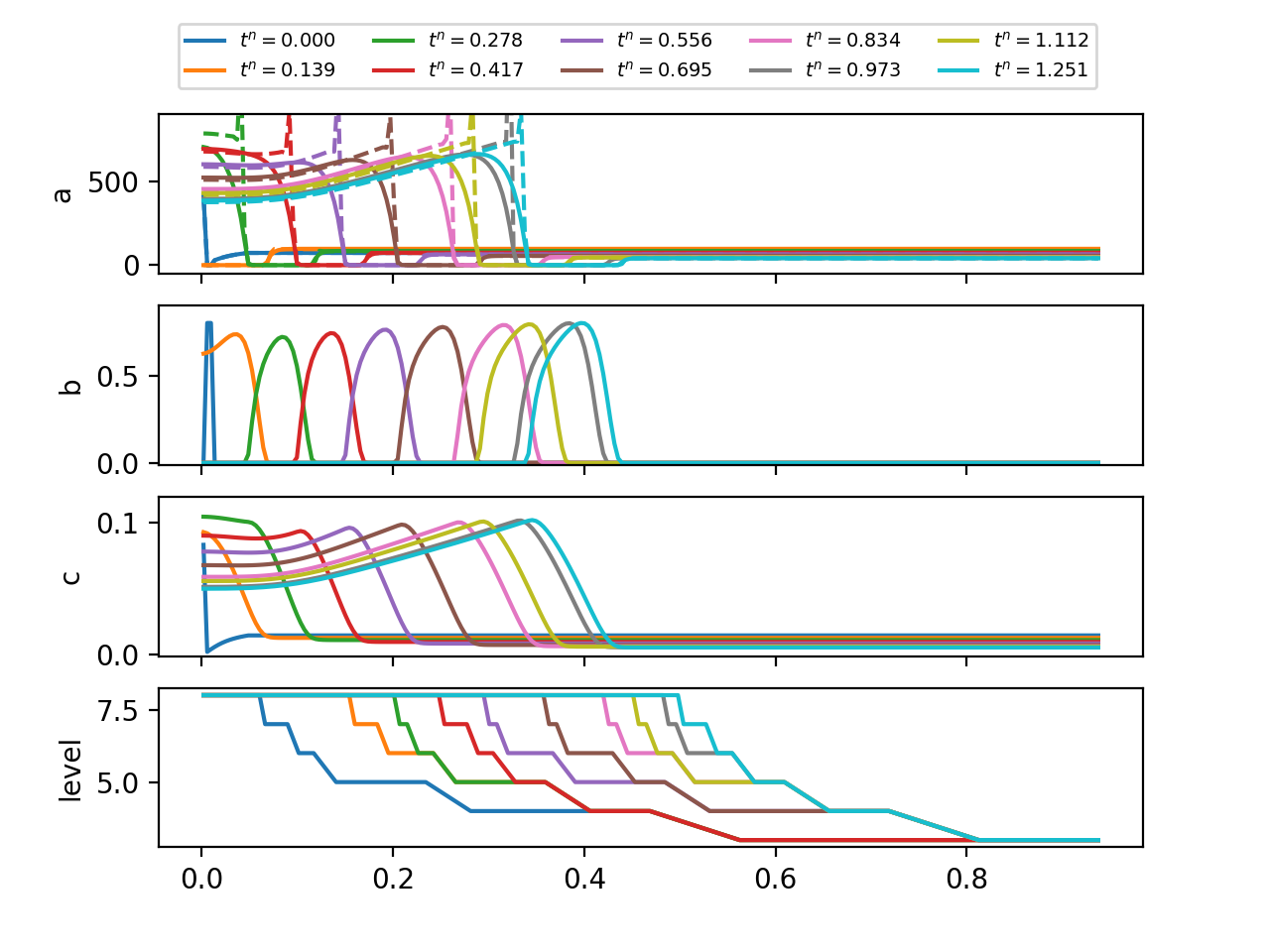
Belousov Zhabotinsky

This example needs to activate -DBUILD_SAMURAI_DEMOS=ON

The Belousov Zhabotinsky reaction is a chemical periodic reaction, in this example we look at a 1D reduction model given by

\[\begin{split}\begin{cases} \partial_t a &= D_a \partial_{xx}a + \frac{1}{\mu}(-qa -ab + fc) \\ \partial_t b &= D_b \partial_{xx}b + \frac{1}{\epsilon}(qa - ab + b(1-b)) \\ \partial_t c &= D_c \partial_{xx}c + b -c \\ \end{cases}\end{split}\]

with parameter

\[\epsilon = 10^{-3},\quad \mu = 10^{-5},\quad f=3,\quad q = 2\cdot 10^{-4}\]

and diffusion coefficients

\[D_a = \frac{1}{400},\quad D_b = \frac{1}{400},\quad D_c = \frac{0.6}{400}\]

In this example we coupling the mesh refinement library samurai with ponio, and the system is solved by PIROCK method.

Belousov Zhabotinsky system solved by PIROCK method

All example in belousov_zhabotinsky_pirock.cpp, and run

make belousov_zhabotinsky_pirock_visu

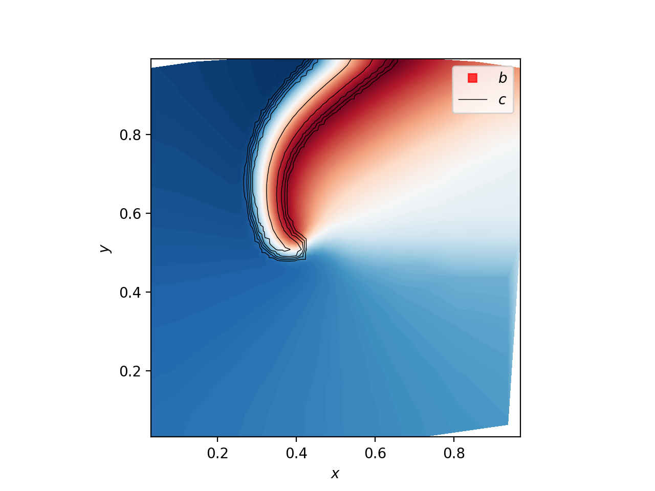
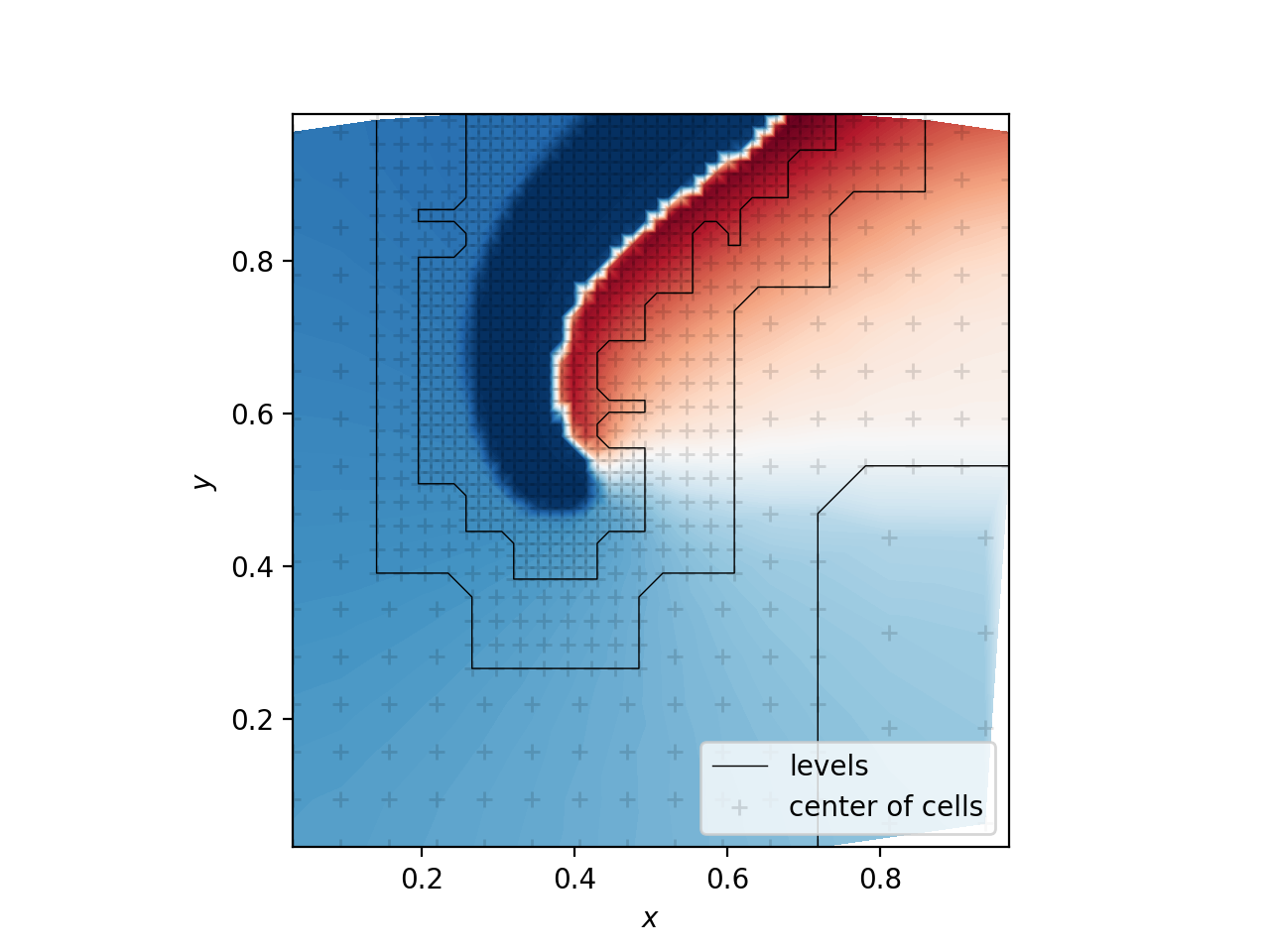
Belousov Zhabotinsky in 2D

This example needs to activate -DBUILD_SAMURAI_DEMOS=ON

The Belousov Zhabotinsky reaction is a chemical periodic reaction, in this example we look at a 1D reduction model given by

\[\begin{split}\begin{cases} \partial_t a &= D_a \Delta a + \frac{1}{\mu}(-qa -ab + fc) \\ \partial_t b &= D_b \Delta b + \frac{1}{\epsilon}(qa - ab + b(1-b)) \\ \partial_t c &= D_c \Delta c + b -c \\ \end{cases}\end{split}\]

with parameter

\[\epsilon = 10^{-2},\quad \mu = 10^{-5},\quad f=1.6,\quad q = 2\cdot 10^{-3}\]

and diffusion coefficients

\[D_a = 2.5\cdot 10^{-3},\quad D_b = 2.5\cdot 10^{-3},\quad D_c = 1.5\cdot 10^{-3}\]

In this example we coupling the mesh refinement library samurai with ponio, and the system is solved by PIROCK method.

Solution \(b\) and \(c\)	Levels of adapted mesh on solution

All example in bz_2d_pirock.cpp, and run

make bz_2d_pirock_visu