Curtiss and Hirschfelder problem

We would like to solve the folowing problem:

\[\begin{split}\begin{cases} \dot{y} = k(\cos(t) - y)\\ y(0) = y_0 \end{cases}\end{split}\]

with \(k>1\), a parameter that allows to control the stiffness of the problem.

%system mkdir -p curtiss_hirschfelder_demo

[]

%%writefile curtiss_hirschfelder_demo/main.cpp

#include <iostream>
#include <valarray>

#include "ponio/solver.hpp"
#include "ponio/observer.hpp"
#include "ponio/problem.hpp"
#include "ponio/runge_kutta.hpp"

int main()
{
    using namespace ponio::observer;

    double k = 50.0;

    double L = -k;
    auto N = ponio::make_simple_problem([=]( double t, double const& u ) {
        return k*std::cos(t);
    });
    auto pb  = ponio::make_lawson_problem(L, N);

    double dt = 0.05;
    double tf = 2;
    double y_ini = 2.0;

    auto exp = [](double x){ return std::exp(x); };

    auto jac = [&]( double t, double const& u ) {
        return -k;
    };

    auto ipb = ponio::make_implicit_problem( pb, jac );

    ponio::solve(pb, ponio::runge_kutta::rk_44()              , y_ini, {0.,tf}, dt, "curtiss_hirschfelder_demo/sol_rk44.dat"_fobs);
    ponio::solve(pb, ponio::runge_kutta::lrk_44(exp)          , y_ini, {0.,tf}, dt, "curtiss_hirschfelder_demo/sol_lrk44.dat"_fobs);
    ponio::solve(pb, ponio::runge_kutta::hochbruck_ostermann(), y_ini, {0.,tf}, dt, "curtiss_hirschfelder_demo/sol_ho.dat"_fobs);
    ponio::solve(pb, ponio::runge_kutta::exprk22()            , y_ini, {0.,tf}, dt, "curtiss_hirschfelder_demo/sol_exprk22.dat"_fobs);
    ponio::solve(ipb, ponio::runge_kutta::backward_euler()    , y_ini, {0.,tf}, dt, "curtiss_hirschfelder_demo/sol_be.dat"_fobs);
    ponio::solve(ipb, ponio::runge_kutta::lsdirk43()          , y_ini, {0.,tf}, dt, "curtiss_hirschfelder_demo/sol_lsdirk43.dat"_fobs);

    return 0;
}

Writing curtiss_hirschfelder_demo/main.cpp

%system $CXX -std=c++20 -I ../include curtiss_hirschfelder_demo/main.cpp -o curtiss_hirschfelder_demo/main

[]

%system ./curtiss_hirschfelder_demo/main

[]

import numpy as np
import matplotlib.pyplot as plt

y0 = 2.0
t0 = 0.0
k = 50.0

def sol(t):
    c0 = (y0 - k/(k**2+1)*( k*np.cos(t0) + np.sin(t0) ))*np.exp(-k*t0)
    return k/(k**2+1)*(k*np.cos(t) + np.sin(t)) + c0*np.exp(-k*t)

time = np.linspace(0, 2, 100)
exact_sol = sol(time)

methods = {
    'rk44': "RK(4,4)",
    'lrk44': "Lawson RK(4,4)",
    'ho': "Hochbruck-Ostermann",
    'exprk22': "expRK(2,2)",
    'be': "Backward Euler",
    'lsdirk43': "L-SDIRK-43"
}

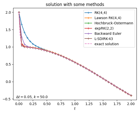
for key, val in methods.items():
    data = np.loadtxt(f"curtiss_hirschfelder_demo/sol_{key}.dat")
    t = data[:, 0]
    y = data[:, 1]

    plt.plot(t, y, "+-", label=val)

plt.plot(time, exact_sol, "--", label="exact solution")

plt.xlabel("$t$")
plt.title("solution with some methods")
plt.text(plt.xlim()[0] + 0.05,plt.ylim()[0] + 0.05, r"$\Delta t = {}$, $k={}$".format(data[0,-1], k))
plt.legend()
plt.show()

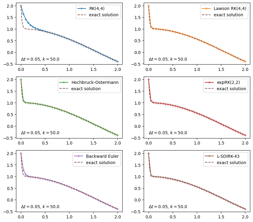
fig, axs = plt.subplots(ncols=2, nrows=len(methods)//2+len(methods)%2, figsize=(10, 3*len(methods)//2))

for i, (key, val) in enumerate(methods.items()):
    data = np.loadtxt(f"curtiss_hirschfelder_demo/sol_{key}.dat")
    t = data[:, 0]
    y = data[:, 1]

    xmin = np.min(t)
    ymin = np.min(y) + 0.05

    axs[i//2, i%2].plot(t, y, "+-", color=f"C{i}", label=val)
    axs[i//2, i%2].plot(time, exact_sol, "--", color="C5", label="exact solution")

    axs[i//2, i%2].text(xmin, ymin, r"$\Delta t = {}$, $k={}$".format(data[0,-1], k))

    axs[i//2, i%2].legend()

plt.show()

def error( t, y ):
    return np.abs( (sol(t) - y) )
def relative_error( t, y ):
    return np.abs( (sol(t) - y)/sol(t) )

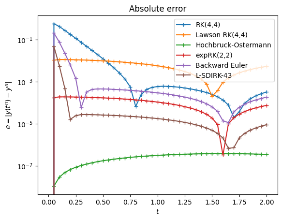
for key, val in methods.items():
    data = np.loadtxt(f"curtiss_hirschfelder_demo/sol_{key}.dat")
    t = data[:, 0]
    y = data[:, 1]

    plt.plot(t, error(t, y), "+-", label=val)

plt.legend()
plt.xlabel("$t$")
plt.ylabel("$e = | y(t^n) - y^n |$")
plt.yscale('log')
plt.title("Absolute error")
plt.show()

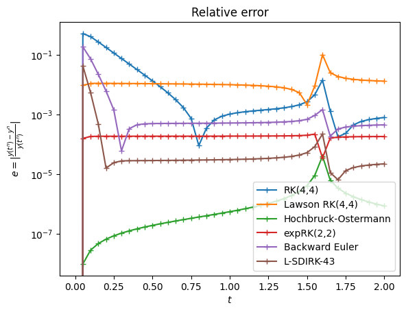
for key, val in methods.items():
    data = np.loadtxt(f"curtiss_hirschfelder_demo/sol_{key}.dat")
    t = data[:, 0]
    y = data[:, 1]

    plt.plot(t, relative_error(t, y), "+-", label=val)

plt.legend()
plt.xlabel("$t$")
plt.ylabel("$e = \\left| \\frac{y(t^n) - y^n}{y(t^n)} \\right|$")
plt.yscale('log')
plt.title("Relative error")
plt.show()