Lotka-Volterra system with a Runge-Kutta method

In this example we present how to write a program to solve the Lotka-Volterra equations with Ponio.

The system is definied as:

\[\begin{split}\begin{aligned} \frac{\mathrm{d}x}{\mathrm{d}t} &= \alpha x - \beta xy \\ \frac{\mathrm{d}y}{\mathrm{d}t} &= \delta xy - \gamma y \\ \end{aligned}\end{split}\]

where:

• \(x\) is the number of prey

• \(y\) is the number of predators

• \(t\) represents time

• \(\alpha\), \(\beta\), \(\gamma\) and \(\delta\) are postive real parameters describing the interaction of the two species.

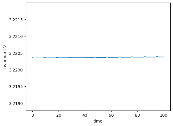
We would like to compute the invariant \(V\) definied by:

\[V = \delta x - \gamma \ln(x) + \beta y - \alpha \ln(y)\]

Define the state

In Ponio is build to solve a problem defined as:

\[\dot{u}(t) = f(t,u(t))\]

we defined as a state (or state_t) the type which represents \(u\). In scalar problems, state_t is often double. In system problems, state_t has multiple composants and Ponio need to make some arithmetic operations on it, so it can be a `std::valarray<double> <https://en.cppreference.com/w/cpp/numeric/valarray>`__ or Eigen vector, etc.

For Lotka-Volterra we have 2 composants so we will use in this example std::valarray<double>. We can defined this as:

using state_t = std::valarray<double>;

Define problem

The `ponio::solve <#>`__ function take as first argument a problem. In Ponio, a problem is a invokable object that take two arguments: \(t\) the current time, and \(u\) the current solution. So a problem can be:

• a simple function

• a lambda function

• a functor

• a `ponio::problem <#>`__ (which need an invokable object)

A problem represents function \(f\) in \(\dot{u}=f(t,u)\) ODE. We would like to change easly parameter so we will use a functor (a class that overload () operator):

#include <valarray>

class Lotka_Volterra
{
    using state_t = std::valarray<double>;

    double alpha;
    double beta;
    double gamma;
    double delta;

    public:

    Lotka_Volterra(double a, double b, double g, double d)
    : alpha(a), beta(b), gamma(g), delta(d)
    {}

    state_t
    operator() (double tn, state_t const& un)
    {
        double x = un[0], y = un[1];
        double dx = alpha*x - beta*x*y;
        double dy = delta*x*y - gamma*y;
        return {dx,dy};
    }
};

Simple example

If we would like to save all iterations into a file we can use a observer::file_observer, if we would like to display all into std::cout we can use observer::cout_observer. In this example we print all into a file.

int main()
{
    using state_t = std::valarray<double>;
    using namespace observer;

    double alpha = 2./3., beta=4./3., gamma=1., delta=1.;
    auto pb  = Lotka_Volterra(alpha,beta,gamma,delta);

    double dt = 0.1;
    double tf = 100;
    state_t u_ini = {1.8,1.8};

    ponio::solve(pb, ponio::runge_kutta::rk_44<>(), u_ini, {0.,tf}, dt, "lv1.dat"_fobs);

    return 0;
}

Where ponio::runge_kutta::rk_44<>() create an instance of algorithm to solve the problem, which represent classical RK(4,4) method.

%system mkdir -p lotka_volterra_rungekutta_demo

[]

%%writefile lotka_volterra_rungekutta_demo/main.cpp

#include <iostream>
#include <valarray>

#include "ponio/solver.hpp"
#include "ponio/observer.hpp"
#include "ponio/runge_kutta.hpp"

class Lotka_Volterra
{
    using state_t = std::valarray<double>;

    double alpha;
    double beta;
    double gamma;
    double delta;

    public:

    Lotka_Volterra(double a, double b, double g, double d)
    : alpha(a), beta(b), gamma(g), delta(d)
    {}

    void
    operator() (double tn, state_t const& un, state_t& dun)
    {
        double x = un[0], y = un[1];
        double dx = alpha*x - beta*x*y;
        double dy = delta*x*y - gamma*y;

        dun[0] = dx;
        dun[1] = dy;
    }
};

int main()
{
    using state_t = std::valarray<double>;
    using namespace ponio::observer;

    double alpha = 2./3., beta=4./3., gamma=1., delta=1.;
    auto pb  = Lotka_Volterra(alpha,beta,gamma,delta);

    double dt = 0.1;
    double tf = 100;
    state_t u_ini = {1.8,1.8};

    ponio::solve(pb, ponio::runge_kutta::rk_44(), u_ini, {0.,tf}, dt, "lotka_volterra_rungekutta_demo/rk_44.dat"_fobs);

    return 0;
}

Writing lotka_volterra_rungekutta_demo/main.cpp

%system $CXX -std=c++20 -I ../include lotka_volterra_rungekutta_demo/main.cpp -o lotka_volterra_rungekutta_demo/main

[]

%system ./lotka_volterra_rungekutta_demo/main

[]

import numpy as np
import matplotlib.pyplot as plt

data = np.loadtxt("lotka_volterra_rungekutta_demo/rk_44.dat")
t = data[:,0]
x = data[:,1]
y = data[:,2]

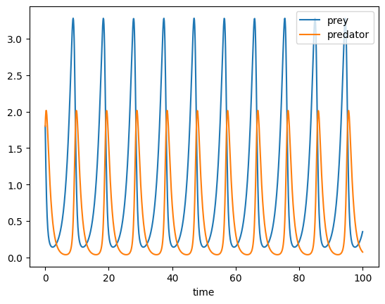
plt.plot(t,x,label="prey")
plt.plot(t,y,label="predator")
plt.xlabel("time")
plt.legend()
plt.show()

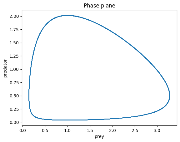
plt.plot(x,y)
plt.xlabel("prey")
plt.ylabel("predator")
plt.title("Phase plane")
plt.show()

Now define the invariant \(V\) :

\[V = \delta x - \ln(x) + \beta y - \alpha \ln(y)\]

def V(x,y, alpha=2./3., beta=4./3., gamma=1., delta=1.):
    return delta*x - np.log(x) + beta*y - alpha*np.log(y)

plt.plot(t,V(x,y))
plt.xlabel("time")
plt.ylabel("invanriant $V$")
vmax = max(V(x,y))
plt.ylim([(1-5e-4)*vmax,(1+5e-4)*vmax])
plt.show()