Lotka-Volterra system with a Lawson method

In this example we reuse previous definition in Lotka-Voleterra resolution with Runge-Kutta method which is the first tutorial. In this notebook we solve the same example.

The system is definied as:

\[\begin{split}\begin{aligned} \frac{\mathrm{d}x}{\mathrm{d}t} &= \alpha x - \beta xy \\ \frac{\mathrm{d}y}{\mathrm{d}t} &= \delta xy - \gamma y \\ \end{aligned}\end{split}\]

where:

• \(x\) is the number of prey

• \(y\) is the number of predators

• \(t\) represents time

• \(\alpha\), \(\beta\), \(\gamma\) and \(\delta\) are postive real parameters describing the interaction of the two species.

We would like to compute the invariant \(V\) definied by:

\[V = \delta x - \gamma \ln(x) + \beta y - \alpha \ln(y)\]

Lawson methods

Lawson methods are a class of time integration schemes that are applied to differential equations of the form:

\[\dot{u} = Lu + N(t,u), \qquad u(t=0) = u_0\]

where \(L\) is a matric and \(N:(t,u)\mapsto N(t,u)\) is a, in general nonlinear, function of the unknow \(u\), and the time \(t\geq 0\). Lawson methods are especially efficient when applied to problems where \(L\) implies a stringent stability condition if it is treated explicitly. Solving this equation with a Lawson method relies of the following change of variable:

\[v(t) := e^{-tL}u(t)\]

Plugging this into our equation yields

\[\dot{v} = e^{-tL}N(t,e^{tL}v)\]

Now an explicit Runge-Kutta method is applied to the transformed equation. We introduce the time discretization \(t^n = n\Delta t\) with \(\Delta t>0\) the time step, \(n\in\mathbb{N}\) and \(u^n\) (respectivement \(v^n\)) denotes the numerical approximation of \(u(t^n)\) (resp. \(v(t^n)\)). For the sake of simplicity, we first present the method for the explicit Euler scheme. Applying the forward Euler method to this problem leads to

\[v(t^n+\Delta t)\approx v^{n+1} = v^n + \Delta t e^{-t^nL}N(t^n, e^{t^nL}v^n)\]

Reversing the change of variable \(u(t) = e^{tL}v(t)\) yields the following scheme for \(u^n\)

\[u(t^n+\Delta t)\approx u^{n+1} = e^{\Delta t L}u^n + \Delta t e^{\Delta tL}N(t^n, u^n)\]

This is the Lawson-Euler method, also a method of order one. More generally, the Lawson method induced by an explicit Runge-Kutta method RK(\(s\),\(p\)) with \(s\) stages of order \(p\) can be written as:

\[\begin{split} \begin{aligned} k_i &= e^{-c_i\Delta t L}N(t^n + c_i\Delta t, e^{c_i\Delta tL}(u^n + \Delta t\sum_{j=1}^s a_{ij}k_j)\\ u^{n+1} &= e^{\Delta tL}(u^n + \Delta t\sum_{i=1}^s b_ik_i) \end{aligned}\end{split}\]

Here, we defined the following linear and non linear part:

\[\begin{split}L = \begin{pmatrix} \alpha & 0 \\ 0 & -\gamma \end{pmatrix}, \qquad N:(t,u)\mapsto \begin{pmatrix} -\beta xy \\ \delta xy \end{pmatrix}\end{split}\]

Ponio doesn’t provide a general exponential function, nor a matrix data structure, so we recommend to use Eigen. In this case linear part is diagonally so we can only use a std::valarray<double> as other examples.

To keep \(L\) and \(N\) in a same object, Ponio provide a ponio::lawson_problem:

state_t L = {alpha, -gamma};
auto N = [=]( double t, state_t const& un ) -> state_t {
    double x = un[0], y = un[1];
    return { -beta*x*y, delta*x*y };
};

auto pb = ponio::make_lawson_problem(L, N);

This problem pb can be use as a ponio::simple_problem or ponio::problem. If we call ponio::solve with a ponio::lawson_problem and a Lawson algorithm (same name as Runge-Kutta algorithm but prefixed by l) Ponio applies a Lawson method to solve the problem. Calling a Lawson algorithm neeed to provide a exponential function, here we propose a solution with overloading of exponential function for std::valarray.

auto exp = [](state_t const& x)->state_t { return std::exp(x); };
ponio::solve(pb, ponio::runge_kutta::lrk_44<>(exp), u_ini, {0.,tf}, dt, "lv_demo/lv1_lawson.dat"_fobs);

%system mkdir -p lotka_volterra_lawson_demo

[]

%%writefile lotka_volterra_lawson_demo/main.cpp

#include <iostream>
#include <valarray>

#include "ponio/solver.hpp"
#include "ponio/observer.hpp"
#include "ponio/problem.hpp"
#include "ponio/runge_kutta.hpp"

int main()
{
    using state_t = std::valarray<double>;
    using namespace ponio::observer;

    double alpha = 2./3., beta=4./3., gamma=1., delta=1.;

    state_t L = { alpha, -gamma };
    auto N = [=]( double t, state_t const& u, state_t& du ) {
        double x=u[0], y=u[1];
        du[0] = -beta*x*y;
        du[1] = delta*x*y;
    };
    auto pb  = ponio::make_lawson_problem(L,N);

    auto exp = [](state_t const& x)->state_t { return std::exp(x); };

    double dt = 0.1;
    double tf = 100;
    state_t u_ini = {1.8,1.8};

    ponio::solve(pb, ponio::runge_kutta::lrk_44(exp), u_ini, {0.,tf}, dt, "lotka_volterra_lawson_demo/lrk_44.dat"_fobs);

    return 0;
}

Writing lotka_volterra_lawson_demo/main.cpp

%system $CXX -std=c++20 -I ../include lotka_volterra_lawson_demo/main.cpp -o lotka_volterra_lawson_demo/main

[]

%system ./lotka_volterra_lawson_demo/main

[]

import numpy as np
import matplotlib.pyplot as plt

data = np.loadtxt("lotka_volterra_lawson_demo/lrk_44.dat")
t = data[:,0]
x = data[:,1]
y = data[:,2]

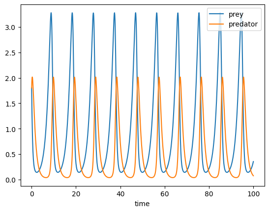
plt.plot(t,x,label="prey")
plt.plot(t,y,label="predator")
plt.xlabel("time")
plt.legend()
plt.show()

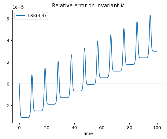
Now define the invariant \(V\) :

\[V = \delta x - \ln(x) + \beta y - \alpha \ln(y)\]

def V(x,y, alpha=2./3., beta=4./3., gamma=1., delta=1.):
    return delta*x - np.log(x) + beta*y - alpha*np.log(y)

V0 = V(x[0],y[0])
plt.plot(t,V(x,y)/V0-1.,label="LRK(4,4)")
plt.axhline(0,0,1,linestyle="--",color="grey",linewidth=1)
plt.title("Relative error on invariant $V$")
plt.xlabel("time")
plt.legend()
plt.show()